SRM 744 Div II - C++ vs Haskell
SRM 744 was held on December 14th, 2018. The original editorial can be found here. I am currently learning Haskell so I decided to solve all tasks in it as well and then compare to my original C++ solutions.
ThreePartSplit - Div 2 Easy
Short problem statement: We are given a half open interval [a, d) which contains n = d - a
elements. We need to divide it into three parts such each of them has at least n div 3 elements.
We need to return the “middle” interval as [b, c) (so half open again).
Solution: A simple and quick task that can be solved analytically, we just need to be
careful not to mess up +-1 indices. There also multiple possible solutions, but maybe the most
straightforward one (at least for me) was to assign n div 3 elements to the first two parts and
then whatever is left to the third part.
E.g. if we were given [0, 8) as a starting interval, that means we have
numbers 0, 1, 2, 3, 4, 5, 6, 7. If we divided them as described above, we’d end up with intervals
[0, 1], [2, 3], [4, 5, 6, 7] where we “crammed” all the extra stuff into the last interval.
There are also other valid solutions, e.g. we could’ve put 3 elements in each interval. So if you are using some editor plugin which compares against the example test cases (like Vimcoder) don’t worry if it reports some of your solutions as wrong.
C++
1
2
3
4
5
6
7
8
class ThreePartSplit
{
public:
    vector <int> split(int a, int d) {
        int minIntervalSize = (d - a) / 3;
        return {a + minIntervalSize, a + 2 * minIntervalSize};
    }
};
It was really cool for me to learn here how we can construct and return vector in a single line, very clean and readable.
Haskell
1
2
3
threePartSplit :: Int -> Int -> (Int, Int)
threePartSplit a d = (a + minIntervalSize, a + 2 * minIntervalSize)
    where minIntervalSize = (d - a) `div` 3
Comparison
| Language | Lines | 100 runs |
|---|---|---|
| C++ | 8 | TBD |
| Haskell | 3 | TBD |
Although Haskell solutions has a bit less lines than C++ one (mostly due to C++ class plumbing),
I would say expresiveness-wise solutions are the same. Since it is O(1) analytical solution, we
don’t need any looping or mapping or data structures, and with this concise way of
creating a vector C++ solution is also very nice to read.
MagicNumbersAgain - Div 2 Medium
Short problem statement: Number is magic if it is a perfect square and if its digits alternate
in a fashion of greater, smaller, greater, smaller, … (e.g. 1 3 2 17 4 2 3). Given [A, B]
interval, find out how many magic numbers it contains.
Solution: The naive solution would be to check for each number between A and B whether it
is a magic number or not. However, due to the constraints (interval can have up to
1010 elements), we can see it would not be fast enough in all the possible cases.
But if we could be a bit smarter and somehow first find all the perfect squares in [A, B] and
then only examine them instead of every number in the interval, would that be more performant?
Sure it would, and since we will need to examine at most 105 squares
(since 105 hits the upper range bound when squared), we can be sure it is going to
be fast enough.
Finding squares is also not a problem, we can just keep iterating over the roots and generate them until we go over the upper range bound.
C++
1
2
3
4
5
6
7
8
9
10
11
12
13
14
15
16
17
18
19
20
21
22
23
24
25
26
27
28
29
30
31
32
33
34
35
36
37
38
39
40
class MagicNumbersAgain
{
public:
    bool isMagic(long long num) {
        // Obtain digits of a number.
        vector<int> digits;
        while (num > 0) {
            digits.push_back(num % 10);
            num /= 10;
        }
        reverse(digits.begin(), digits.end());

        // Perform the check on the digits.
        for (int i = 1; i < digits.size(); i++) {
            if (i % 2 == 1) {
                if (digits[i] <= digits[i - 1]) return false;
            } else {
                if (digits[i] >= digits[i - 1]) return false;
            }
        }
        return true;
    }

    int count(long long A, long long B) {
        // Find all squares in [1, B].
        vector<long long> allSquares;
        for (long long root = 1; root * root <= B; root++) {
            allSquares.push_back(root * root);
        }

        // Check for every square if in [A, B] and magic.
        int magicCount = 0;
        for (int i = 0; i < allSquares.size(); i++) {
            long long square = allSquares[i];
            if (square >= A && square <= B && isMagic(square)) magicCount++;
        }

        return magicCount;
    }
};
A cool trick I learnt here is to generate all the squares from 1 up to B (or even up to the upper limit) and then later just check if it is in the required range. This frees us of doing the work of figuring out what is the first square in the range. Theoretically speaking it is not optimal since we are doing extra work, but here we can afford it and it keeps the code cleaner and less error-prone.
Unfortunately I haven’t used this trick during the competition and made a mistake in just a
situation described above (finding first square >= A) and my solution failed. So it is a good
lesson for the future.
Haskell
1
2
3
4
5
6
7
8
9
10
11
12
13
14
15
16
17
18
19
count :: Int -> Int -> Int
count a b = length $ filter isMagic $ squares a b

squares a b = takeWhile (<=b) $ dropWhile (<a) $ map (^2) [1..]

digits :: Int -> [Int]
digits 0 = []
digits num = digits (num `div` 10) ++ [num `mod` 10]

isMagic :: Int -> Bool
isMagic num = and $ map check triplets
    where
        digs = digits num
        -- Produces (digit, prevDigit, index) triplets.
        triplets = zip3 (drop 1 digs) digs [1..]
        -- Checks whether greater, smaller progression holds.
        check (dig, prevDig, idx)
            | idx `mod` 2 == 1  = dig > prevDig
            | otherwise         = dig < prevDig
Comparison
| Language | Lines | 100 runs |
|---|---|---|
| C++ | 40 | TBD |
| Haskell | 19 | TBD |
I really enjoyed writing this Haskell solution - I love how concise is the count function and how
cleanly it breaks the problem into the subproblems that can be addressed (and tested) separately.
I especially like squares function - how it starts with an infinite list and then we just “trim”
it from the both sides until we get the desired result. This way of thinking makes it much easier
for me to reason and thus much harder to introduce “off-1” type of bugs.
What I find as most different compared to C++ solution is the situation where we have to check the digits, and compare each digit with the previous digit. Since we don’t do looping as in C++ we have to in advance construct all the “checks” with all the information needed.
ModularQuadrant - Div 2 Hard
Short problem statement: We are given an infinite, zero-indexed square grid. Each cell contains
max(row, column) mod 3 value. Given a rectangle in that grid, return the sum of its cells.
Solution: The naive solution would be to go over all the cells in the given rectangle, calculate the values and sum it all together. However, since both width and height of the rectangle can be up to 109, it would be way to slow (we’d need to traverse over 1018 cells in the worst case).
So we need to be smarter and somehow use the properties of this grid to our advantage. Let’s examine the portion of the grid of size 10 x 10:
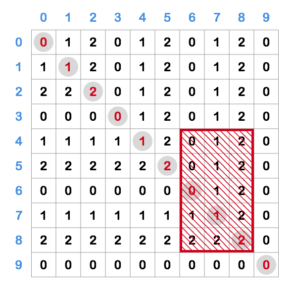
I emphasized the diagonal and the red box is an example of rectangle for which we want to calculate the sum of its cells.
We can notice several things here:
0 1 2pattern repeating itself due tomod 3- The grid is symmetrical in respect to the diagonal (i-th row == i-th column)
My first approach was to calculate sum of each row separately and then sum that. I could calculate
the sum of row in O(1) (observe the patten in a row - number is
repeated until the diagonal and then starts cycling),
but we still have 109 rows so that was too slow (one test case that took
~6s kept failing).
So we need to be even smarter than that - if calculating a row in O(1) is possible, is there
also some kind of a rectangle whose sum we could calculate in O(1)?
If we could calculate sum of any rectangle that has upper left corner in 0, 0 fast enough,
that would be great, because then we use that to calculate sum of any rectangle in the
following way:
calcRectSum(r1, r2, c1, c2) = calcRect00Sum(r2, c2) - calcRect00Sum(r2, c1 - 1) -
                              calcRect00Sum(r1 - 1, c2) + calcRect00Sum(r1 - 1, c1 - 1)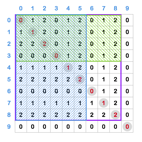
This image should also illustrate what is going on in the formula above (I apologize for the colored mess). If we want to calculate sum of the red box (in the first image) we start with a big purple rectangle and then from it substract the green and blue one. We can see the only thing that is left is what was original a red rectangle. Also, as blue and green rectangles intersect we’ve subtracted that part twice, so we have to add it once to fix that.
That’s it, we’ve managed to express the area of any rectangle with only the rectangles that
start in the 0, 0, upper left corner. So now we only have to find out how to efficiently
calculate sum of such a rectangle (calcRect00Sum method from above).
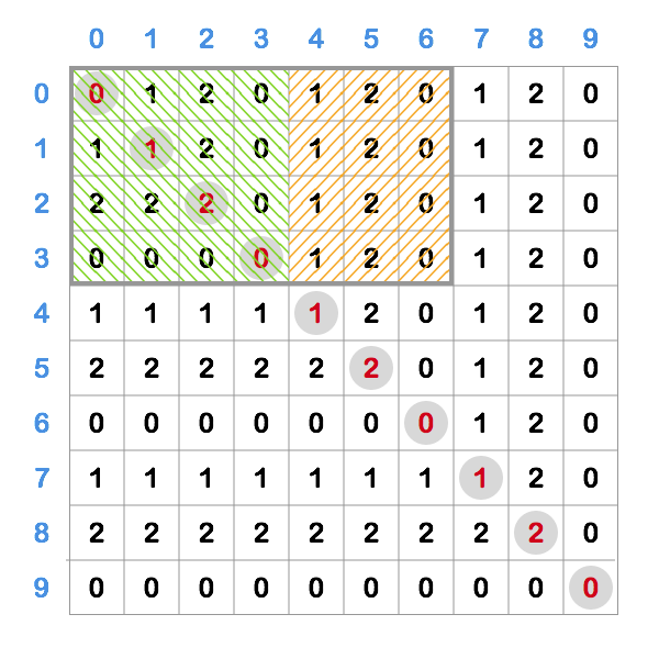
If we look at such a rectangle, we can divide it into two parts - square starting at (0, 0) (green)
and the rest of it (orange).
Calculating a square sum - we can see that numbers are progressing in amount as odd numbers,
1, 3, 5, 7, 9, ... and sum like that we can calculate in O(1) so we can use that.
Let’s take a look at a bit bigger example of a square starting at (0, 0):
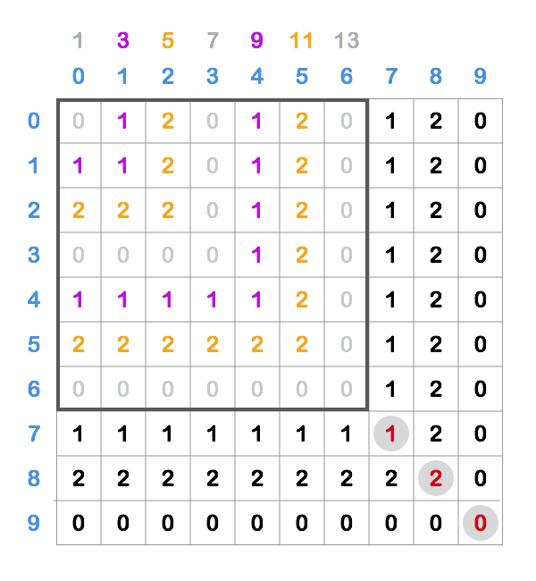
Here we can see that the square consists of “L-shaped” layers (colored in the image) that progress
in the amount of cells as odd numbers (1, 3, 5, 7, ...), which is shown by numbers above the
columns in the image.
We can also see that for a particular value (0, 1, 2) that the number of cells in the layer
progresses by 6 (e.g. first we have 3 1s, than 9, than 15, …) - because of this period of 3,
we have to “skip” two other numbers before coming to the next occurrence of the one that is
observed.
So the sum of the square in the image above can be calculated as:
1
0 * (1 + 7 + 13) + 1 * (3 + 9) + 2 * (5 + 11) = 44
We can generalize that to multiplying each value (0, 1, 2) with a sum of series that starts at
a particular number, has a step of 6 and has number of elements that is equal to the number of
“layers” this value has in the square.
If we can calculate the sum of this series in O(1) (and we can, check the seriesSum method in
the code below), that means this whole calculation is done in O(1), which is exactly what we
were aiming for.
Calculating the rest - we see it has a repeating pattern in a row so we can use that to calculate the sum.
C++
1
2
3
4
5
6
7
8
9
10
11
12
13
14
15
16
17
18
19
20
21
22
23
24
25
26
27
28
29
30
31
32
33
34
35
36
37
38
39
40
41
42
43
44
45
46
47
48
49
50
51
52
class ModularQuadrant
{
public:
    long long seriesSum(int start, int step, int length) {
        int end = start + (length - 1) * step;

        long long sum = (long long)(start + end) * (length / 2);
        if (length % 2 == 1) sum += (start + end) / 2;

        return sum;
    }

    long long calcSquare00Sum(int a) {
        // Number occurrences of 1.
        long long onesOcc = a / 3 + (a % 3 == 2 ? 1 : 0);

        // Number occurrences of 2.
        long long twosOcc = a / 3;

        long long onesSum = seriesSum(3, 6, onesOcc);
        long long twosSum = 2 * seriesSum(5, 6, twosOcc);

        return onesSum + twosSum;
    }

    long long calcRectRightOfDiagonalSum(int startCol, int length, int height) {
        long long rowSum = (length / 3) * (long long)3;

        // Add remainder part.
        int currVal = startCol % 3;
        for (int i = 0; i < (length % 3); i++) {
            rowSum += currVal;
            currVal = (currVal + 1) % 3;
        }

        return rowSum * height;
    }

    long long calcRect00Sum(int r, int c) {
        // The grid is symmetrical so it is the same.
        if (r > c) return calcRect00Sum(c, r);

        return calcSquare00Sum(r + 1) + calcRectRightOfDiagonalSum(r + 1, c - r, r + 1);
    }

    long long sum(int r1, int r2, int c1, int c2)
    {
        return calcRect00Sum(r2, c2) - calcRect00Sum(r2, c1 - 1) - calcRect00Sum(r1 - 1, c2)
            + calcRect00Sum(r1 - 1, c1 - 1);
    }

};
Haskell
1
2
3
4
5
6
7
8
9
10
11
12
13
14
15
16
17
18
19
20
21
22
23
24
25
26
27
28
29
30
31
seriesSum :: Int -> Int -> Int -> Int
seriesSum start step length = (start + end) * (length `div` 2) + middleIfOdd
    where
        end = start + (length - 1) * step
        -- If there is odd number of elements, we have to add a middle element.
        middleIfOdd = if length `mod` 2 == 1 then (start + end) `div` 2 else 0

calcSquare00Sum :: Int -> Int
calcSquare00Sum a = (seriesSum 3 6 onesOcc) + 2 * (seriesSum 5 6 twosOcc)
    where
        onesOcc = a `div` 3 + if a `mod` 3 == 2 then 1 else 0
        twosOcc = a `div` 3

calcRectRightOfDiagonalSum startCol length height = rowSum * height
    where
        rowSum = (length `div` 3) * 3 + remains
        startValue = startCol `mod` 3
        remains = sum $ map (\r -> (startValue + (r-1)) `mod` 3)[1..(length `mod` 3)]

calcRect00Sum :: Int -> Int -> Int
calcRect00Sum r c
    | r > c = calcRect00Sum c r
    | otherwise = calcSquare00Sum (r + 1) + calcRectRightOfDiagonalSum (r + 1) (c - r) (r + 1)

rectSum :: Int -> Int -> Int -> Int -> Int
rectSum r1 r2 c1 c2 = totalRect - leftRect - topRect + intersectRect
    where
        totalRect       = calcRect00Sum r2 c2
        leftRect        = calcRect00Sum r2 (c1 - 1)
        topRect         = calcRect00Sum (r1 - 1) c2
        intersectRect   = calcRect00Sum (r1 -1) (c1 - 1)
Comparison
| Language | Lines | 100 runs |
|---|---|---|
| C++ | 52 | TBD |
| Haskell | 31 | TBD |
Implementing Haskell solution was pretty straightforward to implement from the C++ solution, we already divided the problem nicely into functions so we could just implement them in Haskell.
The Haskell solution is naturally shorter due to more dense syntax, but the logic stayed pretty
much the same. The final function in Haskell solution, rectSum, I had to rename because
sum is a method that comes in Haskell’s standard library.